.jpg)
Visualize Interactively AIM Images Using the k3d Library
Published:
Visualize Interactively AIM Images Using the k3d Library
This notebook is intended to guide you through the process of visualizing and apply basic image processing operations to the AIM images loaded via the vtkbone library. As the vtkbone library is meant for IO operations, a visualization package is outside of the scope of the library. However, we provide information on the usage of a compatible library, k3d, which integrates seamlessly with the vtk image data structure.
Visualization with k3d
To visualize AIM images interactively in Jupyter notebooks, we use the k3d library. This allows for dynamic interaction with the image data, enhancing the analysis and understanding of the images’ features.
%pip install k3d
Import necessary packages
import vtk
from vtk.util import numpy_support
import k3d
import numpy as np
Read the image using vtkbone
Read in the image using vtkbone. If you do not have vtkbone installed follow the tutorial on how to use vtkbone
# Give the path to your AIM file
impath = Path('./data/TRAB_1240.AIM')
segpath = Path('./data/TRAB_1240_SEG.AIM')
We first read the 3D image from an AIM file using the vtkboneAIMReader. The read_image function is decorated with @print_image_info to print the image’s properties (spacing, origin, dimensions, byte format) upon reading.
# decorator that print informations such as spacing, origin, dimensions, byte format
def print_image_info(func):
    @functools.wraps(func)
    def wrapper(*args, **kwargs):
        image = func(*args, **kwargs)
        spacing = image.GetSpacing()
        origin = image.GetOrigin()
        dimensions = image.GetDimensions()
        byte_format = image.GetScalarTypeAsString()

        print("Image Informations:")
        print(f"Spacing: {np.round(spacing, 3)}")
        print(f"Origin: {np.round(origin, 3)}")
        print(f"Dimensions: {dimensions}")
        print(f"Byte Format: {byte_format}")

        return image

    return wrapper
We then define and apply the function read_image() to read the image from the AIM file. Please refer to notebook 01_reading_in_aims for more details on the vtkboneAIMReader.
@print_image_info
def read_image(aim_path: Path):
    """
    Read a 3D image from a file using the vtkboneAIMReader to read a 3D image from a file in the AIM format.

    Parameters:
    aim_path (Path): The path to the AIM file to read.

    Returns:
    vtkImageData: The 3D image read from the file.
    """
    print(f'Reading file: {aim_path}')
    reader = vtkbone.vtkboneAIMReader()
    reader.DataOnCellsOff()
    reader.SetFileName(str(aim_path.resolve()))
    reader.Update()
    return reader.GetOutput()

# execute the function
image = read_image(impath)
image_seg = read_image(segpath)
Visualize the image using k3d
Convert the image to a numpy array
In this conversion step, we return a numpy array containing the informations of the image. VTK images are indexed in the order [x, y, z], while numpy array are indexed in the opposite order [z, y, x]. We therefore need to reverse the order of the dimensions of the image.
def image2np(image):
    # Use python_helpers.vtk_util to convert vtkImageData to numpy array
    imnp = vtkImageData_to_numpy(image)
    # Transpose and flip the array to have the same indexing and direction as the original AIM image
    imnp = np.transpose(imnp, (2, 1, 0))
    imnp = np.flip(imnp, axis=2)
    # Enforce float16 type (best for k3d)
    imnp = imnp.astype(np.float16)
    return imnp

imnp = image2np(image)
imnp_seg = image2np(image_seg)
Get information about the image for visualization
We then want to include some image information in the visualization. We therefore get the spacing, origin, and dimensions of the image to create a transformation matrix that will be used to correctly position the image in the visualization.
# Extract spacing, origin, and dimensions from a vtkImageData object. These are important properties that describe the resolution, position, and physical size of the image.
spacing = image.GetSpacing()
origin = image.GetOrigin()
dimensions = image.GetDimensions()
Generate a transformation matrix for a 3D image. This function takes the spacing, origin, and dimensions of a 3D image and generates a transformation matrix. This matrix can be used to transform the voxel coordinates of the image to world coordinates.
transform_matrix = np.array([
    [spacing[0] * dimensions[0], 0, 0, origin[0]],
    [0, spacing[1] * dimensions[1], 0, origin[1]],
    [0, 0, spacing[2] * dimensions[2], origin[2]],
    [0, 0, 0, 1]
])
In order to decide which range of intensities we want to visualize, plotting the histogram of the image is a good way to get an idea of the distribution of the intensities.
plt.figure(figsize=(10, 5))
plt.hist(imnp.flatten(), bins=100)
plt.title('Histogram of the image')
plt.show()
For instance, the code snippet below takes into account different cases for the type of images that we read. If the image is a native greyscale, then a good vmin to use as a starting point would be vmin = 3000. If the image is a greyscale with a range of intensities, then we can use the minimum intensity as the starting point. If the image is a mask, the minimum intensity would be 0 and the maximum intensity would be 127.
# We take the numpy array representing the image and calculates the minimum and maximum intensity values for that image.
# These values can be used for setting the intensity range when visualizing the image.
# We can also overwrite these or modify them directly in the k3d controls later on.

# Calculate the minimum and maximum intensity values for a numpy array.
intensity_min = np.min(imnp)
intensity_max = np.max(imnp)

if intensity_max > 1:
    vmin = 0.01
    if intensity_max > 127:
        vmin = 3000
vmax = intensity_max
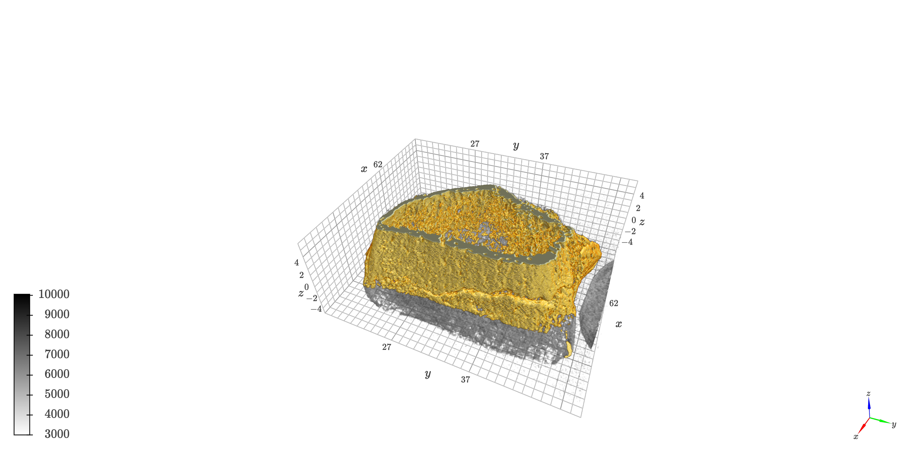
Create the visualization
IMG_SUPERPOSITION = True

transform_s = k3d.transform(custom_matrix=transform_matrix)

# Instantiate the volume plot using k3d-jupyter
plt_volume = k3d.volume(imnp,
                        transform=transform_s,
                        color_map=k3d.colormaps.basic_color_maps.Binary,
                        samples=256,
                        alpha_coef=150,
                        color_range=[vmin, vmax])
plot = k3d.plot()
plot += plt_volume

if IMG_SUPERPOSITION:
    plt_super = k3d.volume(imnp_seg,
                        transform=transform_s,
                        color_map=k3d.colormaps.basic_color_maps.Blues,
                        samples=256,
                        alpha_coef=5,
                        color_range=[0, 1])
    plot += plt_super

# Display the plot inline
plot.display()
Conclusion
This tutorial provides a brief overview of using k3d for interactive visualization of AIM images and introduces basic image processing operations. For more advanced techniques and applications, refer to the other tutorials in this series.